Constraint Programming and
Automatic Differentiation
for Automated Engineering Design
Luke McCulloch, PhD
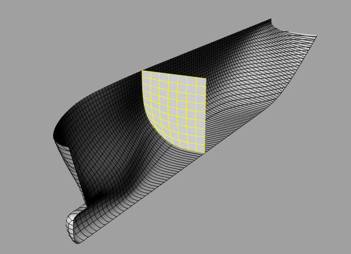
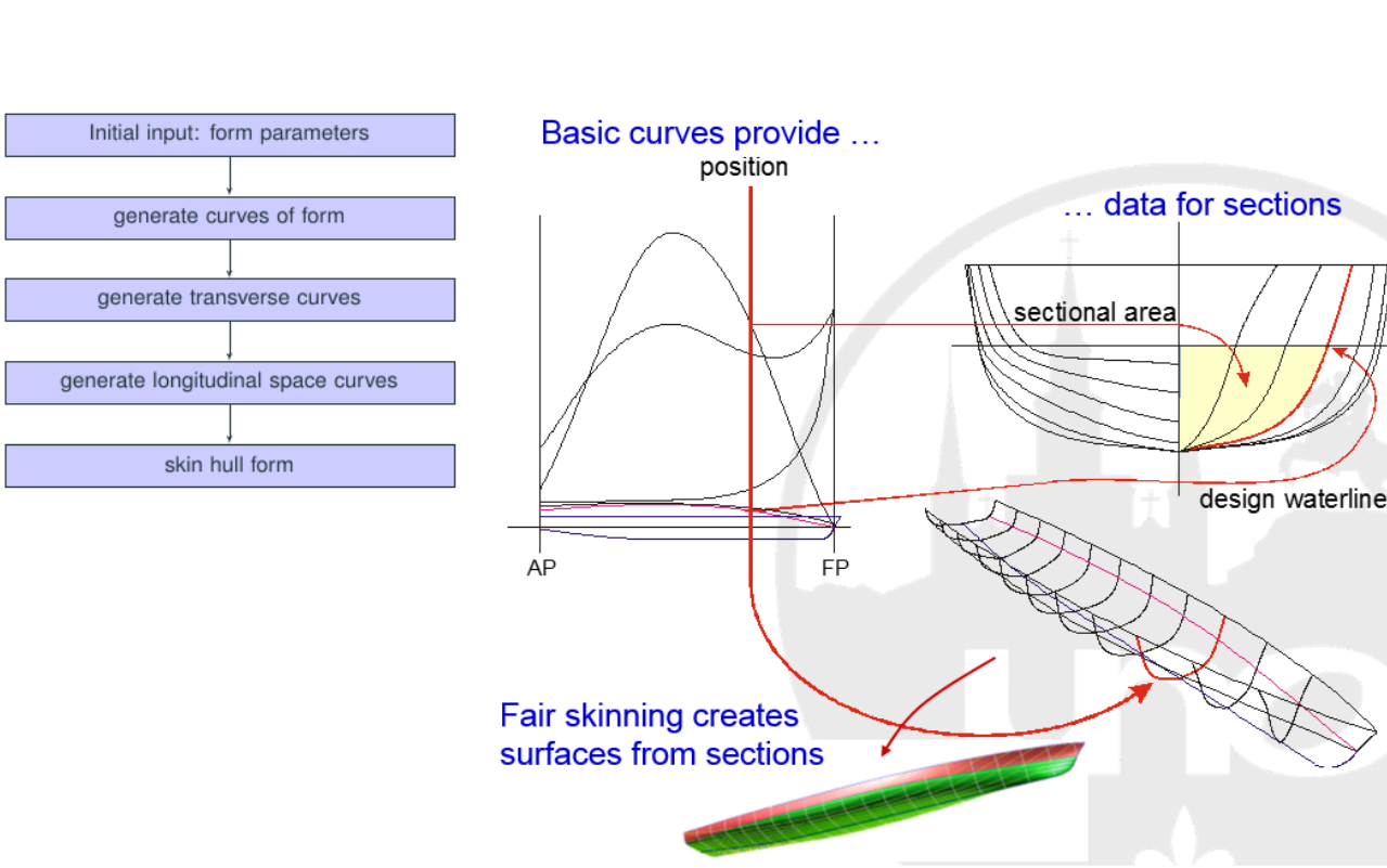
A picked problem: automate the generation of this kind of thing:
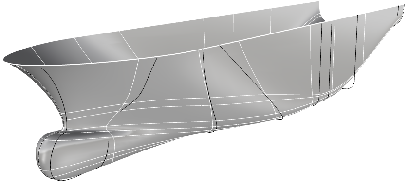
(NURBS early stage hullform (OSV type) in demo in Rhino, human created)
- One of a kind designs
- Less standardization than other industries
- No prototypes, less chance to iron out issues
Use Computation to Reduce Uncertainty
Properties we care about: differential / transitional
Properties we care about: volumetric / represented as area again!
Properties we care about: curvature
Control Properties with: Form Parameter Design
How do we Make a B-spline curve which conforms to constraints?
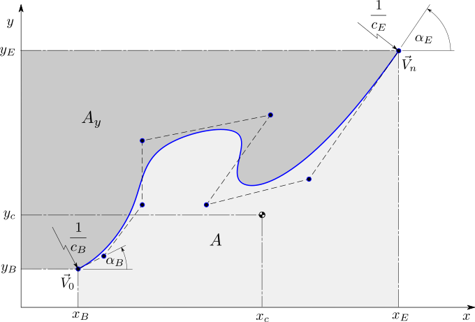
Find a two dimensional open B-spline curve
\begin{equation} \underline{q}(t)\;=\;\sum_{i=0}^{n}\underline{V}_{i}N_{i,k}(t) \label{eq:optproblem} \end{equation}such that a flexible set of selected form parameters, $\underline{h}$ is met and, in addition, the curve is considered "good" in terms of a problem-oriented measure, $f$.
$\underline{V}_{i}$ are the control vertices. These are the free variables in our design.
$N_{i,k}$ are the basis functions
$\underline{q}\left(t\right)$ is the value of the curve at parameter $t$
So, write down the problem:
$$ F = f + \sum_{j \in \left[ \forall h \right]} \lambda_j h_j $$$$ f = f\left(\underline{V}\right) \\ h_j = h_j\left(\underline{V}\right) \\ $$$f$ is a fairness functional to be minimized
$h$ are constraints to be satisfied
$\lambda_j$ are Lagrange multipliers
Solve via Newton's method. (We want geometry that minimizes $F$)
Solution: $\underline{\nabla} F = [0,0,0,0.... ]^T$
Basically find control vertices and Lagrange multipliers such that the gradient of $F$ is zero. (Then check your solution)
What is Automatic Differentiation (AD)?
- no finite differences
- no symbolic derivatives
- values exact to floating point
Derivatives by construction:
- Overload mathmatical operations to return value, gradient, and hessian
- where each computation includes the natural rules from calculus.
(Python Numpy makes it easy to extend to vectors and matrices)
How to setup AD
(assuming you have built a class for the overloading...)
For automatic differentiation on a design space, you need only a couple of matrices:
#Let's say my design space has only 2 variables for the moment

# for the gradient
identity = np.matrix(
                np.identity(2)) # [2x2] identity matrix

# for the Hessian
nullmatrix = np.matrix(
                np.zeros((2,2),float)) # [2x2] null matrix
How to setup AD
Instantiate an AD object:
x0 = ad(0.5,
        grad  = identity[0],
        hess  = nullmatrix)
print 'x0.value = ',x0.value
print 'x0.grad  = ', x0.grad
print 'x0.hess  = '
print x0.hess
How to setup AD
Here is the second variable.
x1 = ad(2.0,
        grad  = identity[1],
        hess  = nullmatrix)

print ''
print 'x1.value = ',x1.value
print 'x1.grad  = ', x1.grad
print 'x1.hess  = '
print x1.hess
Now we are ready to compute something
How about $f = x_0 + x_{1}^{2}$
f = x0 + x1**2

print '\ntest value' # 0.5 + 2**2 = 4 is...?
print f.value

print '\ntest gradient' # df/dx0 , df/dx1 is ..
print f.grad.T

print '\ntest hessian' #[ [df/dx0dx0 ,..., df/dx1dx1]] is ...
print f.hess
B-spline Curves
dimensions = 2   # 2D curve example
order      = 4   #degree + 1

#numpy array:
vertices   = np.asarray([[0.,0.],[2.,0.],[3.0,0.0],[3.0,8.0],
                         [9.0,12.],[11.,12.],[12.,12.]])

curve1 = spline.Bspline(vertices,order) #make Bspline curve
curve1.plotcurve_detailed() #plot it

B-spline properties
A fairness functional objective:
\begin{equation} E_N \;=\; \intop_{t_{B}}^{t_{E}}\left[ \left(\frac{\text{d}^{\text{N}}q_{x}}{\text{dt}^{\text{N}}}\right)^2 \,+\, \left(\frac{\text{d}^{\text{N}} q_y}{\text{dt}^{\text{N}}}\right)^2\,\right] \text{dt} \qquad\text{with $N = 1,2,3$} \end{equation}$E_N$-norms which approximate things with physical analogies. e.g. the bending energy in the curve when $N=2$.
precompute_curve_integrals()
print 'The value of the second fairness functional, E2 is,'
print 'curve1.E2 =', curve1.E2
Automatic Differentation of B-spline Curves
First make AD variables that match the curve vertices:
num_in_vec = len(vertices)
xpts = []
ypts = []
for i in range(num_in_vec):
    xpti = vertices[i,0]
    ypti = vertices[i,1]
    xpts.append( ad( xpti, N=num_in_vec*dimensions,
                    of_scalars=True, dim=i) )
    ypts.append( ad( ypti, N=num_in_vec*dimensions,
                    of_scalars=True, dim=i+num_in_vec) )
How about Auto Diff'ing fairness functionals?
A fairness functional objective:
\begin{equation} E_N \;=\; \intop_{t_{B}}^{t_{E}}\left[ \left(\frac{\text{d}^{\text{N}}q_{x}}{\text{dt}^{\text{N}}}\right)^2 \,+\, \left(\frac{\text{d}^{\text{N}} q_y}{\text{dt}^{\text{N}}}\right)^2\,\right] \text{dt} \qquad\text{with $N = 1,2,3$} \end{equation}$E_N$-norms which approximate things with physical analogies. e.g. the bending energy in the curve when $N=2$.
These can be re-written to pre-compute the integrals.
\begin{equation} E_N \;=\; \; \underline{v}_x^T \cdot \int_{t_B}^{t_E} \underline{\underline{M}}_{N}(t) \text{dt} \cdot \underline{v}_x \,-\, \underline{v}_{y}^T \cdot \int_{t_B}^{t_E} \underline{\underline{M}}_{N}^T(t) \text{dt} \cdot \underline{v}_{y} \end{equation}The $\underline{\underline{M}}_{N}$ are matrices of integrals of prodcts of basis functions and their derivatives which never change.
def fairness(curve, vertices=None):
    """
        Method to compute the non-weighted fairness
        functionals of a B-spline curve.

    """
    if vertices is None:
        xpts = curve.vertices[:,0]
        ypts = curve.vertices[:,1]
    else:
        xpts = vertices[0]
        ypts = vertices[1]
    E1 = np.dot(np.dot(xpts,curve.M1),xpts)+np.dot(np.dot(ypts,curve.M1),ypts)
    E2 = np.dot(np.dot(xpts,curve.M2),xpts)+np.dot(np.dot(ypts,curve.M2),ypts)
    E3 = np.dot(np.dot(xpts,curve.M3),xpts)+np.dot(np.dot(ypts,curve.M3),ypts)

    return E1,E2,E3
These can be re-written to pre-compute the integrals.
\begin{equation} E_N \;=\; \; \underline{v}_x^T \cdot \int_{t_B}^{t_E} \underline{\underline{M}}_{N}(t) \text{dt} \cdot \underline{v}_x \,-\, \underline{v}_{y}^T \cdot \int_{t_B}^{t_E} \underline{\underline{M}}_{N}^T(t) \text{dt} \cdot \underline{v}_{y} \end{equation}The $\underline{\underline{M}}_{N}$ are matrices of integrals of prodcts of basis functions and their derivatives which never change.
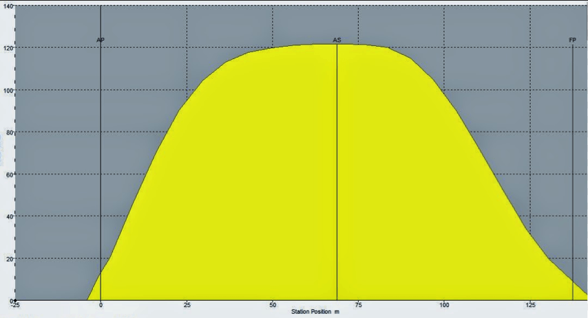
Area integration goes the same way. For that matter, so do moments of area.
#call our new function with AD xpts and ypts:
e1,e2,e3 = fairness(curve1, [xpts,ypts])

print "e2 value = {}".format(e2.value)
print ''
print 'e2 gradient Transposed = '
print e2.grad
How About B-spline Curvature?
\begin{align} c_B \;&=\; \left.\frac{\dot{q}_{x}\ddot{q}_{y} \,-\,\ddot{q}_{x}\dot{q}_{y}}{ \sqrt{\dot{q}_{x}^{2}\,+\,\dot{q}_{y}^{2}}} \right|_{(t=t_{B})} \end{align}Well, you can't pre-compute it efficiently, but it's just products of B-spline derivatives.
AD has no trouble.
In general, we can compute tangents along the curve, arc length, centroids (using moments of area)... many quantities, all analytically.
Let's Optimize this Curve
# create a dictionary to hold components of our Functional F:
FPD = FormParameterDict(curve1)

#fairness functional, f:
FPD.add_E2(kind='LS') # "LS" asks our library to minimize


# now the equality constraints:
#
# C1 (tangent) clamp at the ends:
FPD.add_AngleConstraint(kind='equality', location = 0., value = 0.)
FPD.add_AngleConstraint(kind='equality', location = 1., value = 0.)
#
# C2 curvature clamp at the ends
FPD.add_CurvatureConstraint(kind='equality', location = 0., value = 0.)
FPD.add_CurvatureConstraint(kind='equality', location = 1., value = 0.)

#Setup done.
Let's Optimize this Curve
#setup and solve:
L = Lagrangian(FPD) #shake and bake a bit
Lspline = IntervalLagrangeSpline(curve1, L) #"interval" name is due to history
vertices = Lspline.optimize() #solve it

Lspline.curve.plotcurve_detailed()

Form Parameter Design (FPD) Shortcomings
We optimized that curve. Now we have the basics of FPD.
We used Automatic Differentation to make implementation easy
What's wrong with our automation now?
Even if all of the initially given form requirements are met, there are sometimes flaws in the resulting shapes because the form parameters may not be appropriately attuned to start with. It takes judgment and often some iteration in order to harmonize all requirements.
Computational Geometry for Ships, Nowaki, et al., 1995
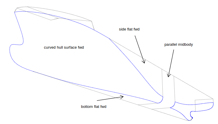
How do we harmonize this?
When our inputs look like this:
(Interval) Constraint Programming
A designer knows he has achieved perfection not when there is nothing left to add, but when there is nothing left to take away.
-Antoine de Saint-Exupéry
How to determine what to take away?
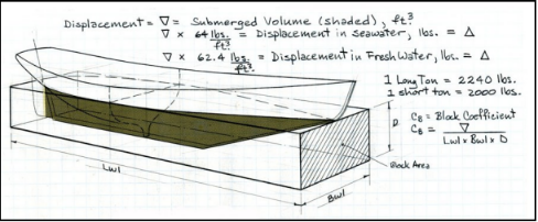
Use Natural Naval Archecture Design Relationships...
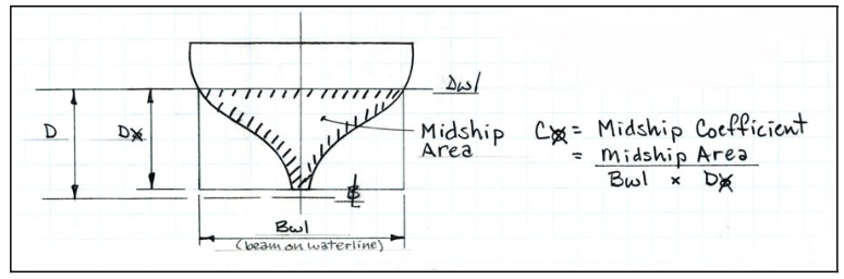
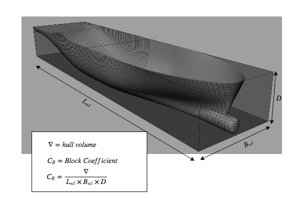
Block Coefficient $$ \text{C}_{\text{B}} = \frac{\nabla}{\text{L}_{\text{WL}} \times \text{B} \times \text{D}} $$ Midship Coefficient $$ \text{C}_{\text{M}} = \frac{\text{A}_{\text{M}}}{\text{B} \times \text{D}} $$ Prismatic Coefficient $$ \text{C}_{\text{P}} = \frac{\nabla}{\text{L}_{\text{WL}} \times \text{B} \times D \times \text{C}_{\text{M}}}= \frac{\text{C}_{\text{B}}}{\text{C}_{\text{M}} } $$
And many others. In fact this framework you can invent your own.
- instead of controlling one number directly as a constraint,
- we specify relationships between the design variables,
- and use constraint solving to eliminate infeasible choices
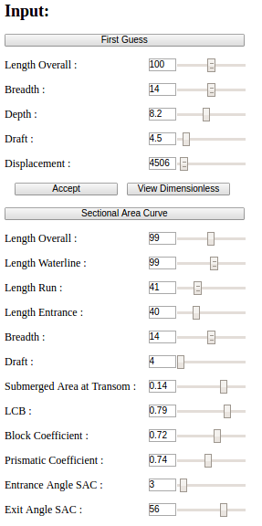
A design space consists of several form parameters:
$$ \begin{eqnarray*} \nabla & : & \text{volumetric displacement} \\ \text{L}_{\text{WL}} & : & \text{length along the waterline} \\ \text{B} & : & \text{width at midship} \\ \text{D} & : & \text{distance from waterline to the keel} \\ \text{A}_{\text{M}} & : & \text{midship area} \\ \text{C}_{\text{B}} & : & \text{block coefficient} \\ \text{C}_{\text{M}} & : & \text{midship coefficient} \end{eqnarray*} $$(in general on the order of 20-30 parameters and design ratios)
Find a form parameter, interval valued, thin, $\textit{ design space}$, $\text{S}$
\begin{equation} S_{j}=[\underline{S_{j}},\overline{S_{j}}] \end{equation}such that all constraints and relations are feasible, and the form parameter design program returns a valid hull geometry.
What am I talking about?
2 Philosophical Choices:
- From single design to operating on the entire design space at once
- via Interval arithmetic (that surely needs explaining)
- How to solve this system of rules (interval equations)
- Matrix of linear equations?
- Local consistencies? (constraint programming)
We choose local consistencies for the technical reason that matrix interval methods often need local consistencies anyway.
Interval Arithmetic, briefly considered.
Interval Arithmetic, in one slide
$$ \left(1.,2.\right) +\left(0.,5.\right) = \left( 1., 7. \right) $$- It's based on closed intervals of real numbers.
- e.g. $\left(1.,2.\right)$ defines a continuum from $1.$ to $2.$ inclusive.
- Operations composed of intervals and bound the range of corresponding real operations, rigorously, using outward rounding, on real computer hardware.
Note: update of old data by new proceeds by taking the intersection.
This is absolutely essential interval constraint and interval optimization, programming.
a = ia(1.,2.)
b = ia(0.,5.)
c = ia(-1000.,1000.)
c = c & (a+b)
print 'c = ',c

c = ia(-2.,3.)
c = c & (a+b)
print 'c = ',c
How do we use an interval valued rule to eliminate infeasible designs?
Interval Constraint programming.
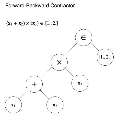
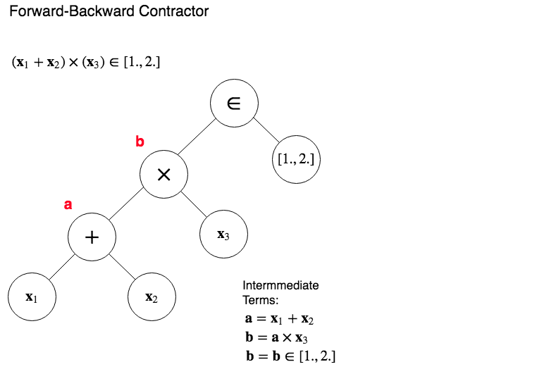
Forward Backward Constraint Propagation
Let's show how a forward backward algorithm works using a simple mathematical expression: $$ \left(x_{1} + x_{2}\right) \times x_{3} \in \left[1.,2.\right] $$
Build the syntax tree
Forward Backward Contractor, Intermediate Terms:
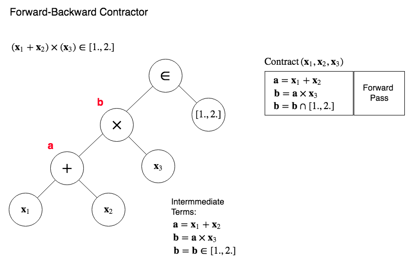
Forward Backward Contractor, Forward Pass:
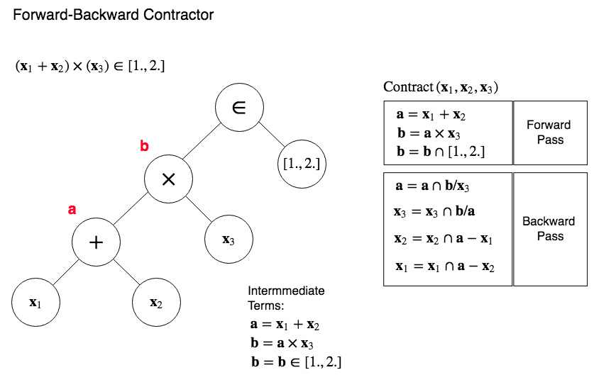
Forward Backward Contractor, Backward Pass:
How do we make it work for arbitrary systems of rules?
Unification
Is an algorithm for making two things equal. (within an environment)
Data can flow in either direction across the equals sign.
fragment= \
"""
def unify(self, a, b):
    ivars = a,b # a and b are logical variables, now saved in ivars
    a = self.value_of(a) # get the value of a
    b = self.value_of(b) # get the value of b
    #...
    if isinstance(a, ia) and isinstance(b, ia):
        values = copy.copy(self.values) # self.values maps vars to values
        # this is the "environment"
        values[ivars[0]] = a & b
        values[ivars[1]] = values[ivars[0]] & b
    #...
"""
Issue: unification always acts on 2 terms.
How do we make logical constraint relations work for any mathmatical statement?
Answer: Compile mathmatical expressions into syntax trees
Use operator overloading to build a tree of relational terms from a mathmatical expression.
- Operator overloading handles parsing of n-ary mathematical terms into ternary constraints.
- The overloading class must Store
- the ternary elements of a computation
- Also store the operation used to combine two of them into the other
- Then we methodically convert those ternary constraints into binary logical rules and perform unification on them.
- We keep track of what terms are used in what rules.
Data can then flow freely between our terms and across rules
This is constraint logic programming.
Let's look at an example design space and see what a rule looks like
"""Make some design space variables:
"""
lwl = lp.PStates(name='lwl')
bwl = lp.PStates(name='bwl')
draft = lp.PStates(name='draft')
vol = lp.PStates(name='vol')
disp = lp.PStates(name='disp')

Cb = lp.PStates(name='Cb')
Cp = lp.PStates(name='Cp')
To make it a real interval desgin space,
vol = vol == ia(50000.,100000.)
bwl = bwl == ia(25.,30.)

#etc
Let's see what a rule syntax tree looks like
"""-----------------------------------------------
#rule: block coefficient
"""
Cb = Cb == vol/(lwl*bwl*draft)

print Cb
Python automatically creates temporaries so that all operators act to combine two terms into a third.
This let's us walk the tree in reverse to compile logical rules.
We keep track of what terms are used in what rules.
Constraints are Compiled Into a Graph:
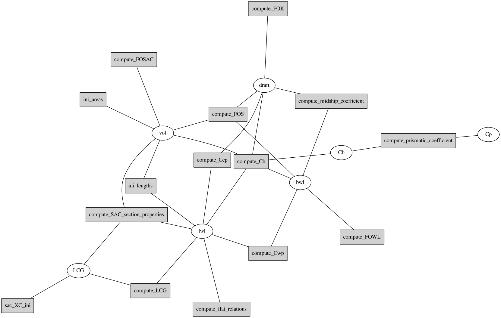
How do we get a single boat out of it?
Select numbers at random, from the feasible domain
- Iterate over the design space one variable at a time
- Pick a number from the feasible domain at random
- Use constraint propagation to update all the other design variables with the new data.
(This eliminates swaths of the design space each time) - Once a single design is determined, do form parameter design.
Resultant hull constraint combinations were always feasible
This made it easy to have form parameter design solve for a decent looking hull
Resulting solved curve form parameters had little error
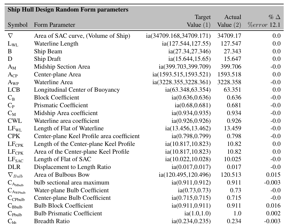
However, by the time the surface is generated, the fit is no longer prefect (future work!)
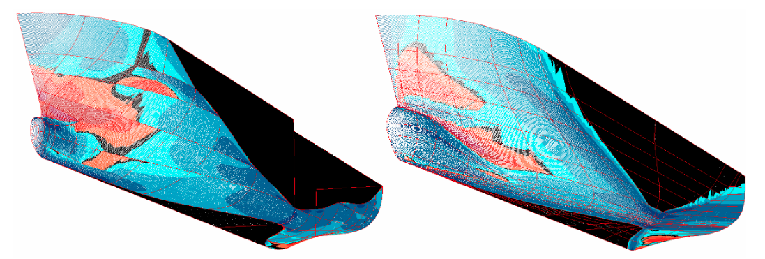
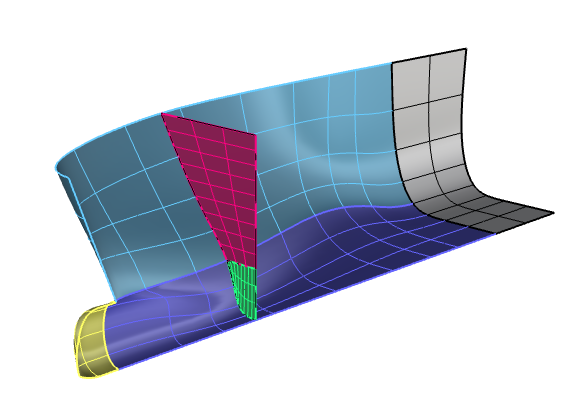
Details: I used spatial splitting (and THB-splines) for fine grained form paremter design
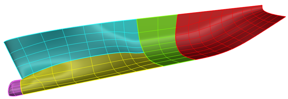
Details: Together with Auto Diff, this allowed much freedom to sculpt interfaces between surface
But I am not using form parameter design to it's fullest.
I focused on making it easier to use.
Thank you for your attention!
Any questions?